By the end of this tutorial, you will know about:

1. What is a Decision Tree?
2. What is ID3?
3. Some vital principles of Decision Tree Learning
4. Build a Decision Tree using ID3 with source code

What is a Decision Tree?

Before a theoretical understanding of what's all about these "Decision Trees", let's first understand what are trees. And what is its structure? Trees have many analogies in real life as they do cover a wider area in the field of Machine Learning. Coming to what's all about "Decision", it is the basic kind of judgment we take given a set of conditions. And that sums up a wide view of what are Decision Trees.

In decision analysis, a decision tree can be used to visually and explicitly represent decisions and decision-making. As the name goes, it uses a tree-like model of decisions.

In layman's terms, or to give a very broad view of what happens in a Decision Tree, it undergoes a continuous split of attributes based on certain parameters till it reaches the end where it cannot split. And that is why, we refer to them as trees, because of the splits we have, they are divided into branches & sub-branches (also called nodes) and from these nodes, there will be a state where the decision is taken. At it point in time, you need not go into the details, if you understand this very process, you are on par with moving on with this blog.

However, if you wish to know much deeper about Decision Trees, you will have a clear understanding in simple terms here in this blog:

What is ID3?

ID3 stands for Iterative Dichotomiser 3 and is named such because the algorithm iteratively (repeatedly) dichotomizes(divides) features into two or more groups at each step. This kind of suits par with the concept of Decision Trees right? wherein we use a repeated division of splits (attributes) to arrive at a conclusion.

So, why not use this ID3 algorithm in the concept of Decision Tree Learning?
Most generally ID3 is only used for classification problems with nominal features only. But let's try developing this algorithm on Iris Dataset

Dataset Description:

Iris Data:

 sepal_length  sepal_width  petal_length  petal_width    species

0             5.1          3.5           1.4          0.2     setosa
1             4.9          3.0           1.4          0.2     setosa
2             4.7          3.2           1.3          0.2     setosa
3             4.6          3.1           1.5          0.2     setosa
4             5.0          3.6           1.4          0.2     setosa
..            ...          ...           ...          ...        ...
145           6.7          3.0           5.2          2.3  virginica
146           6.3          2.5           5.0          1.9  virginica
147           6.5          3.0           5.2          2.0  virginica
148           6.2          3.4           5.4          2.3  virginica
149           5.9          3.0           5.1          1.8  virginica

[150 rows x 5 columns]

Metrics in the ID3

The ID3 algorithm selects the best feature at each step while building a Decision tree. Before you ask, the answer to the question: ‘How does ID3 select the best feature?’ is that ID3 uses Information Gain or just Gain to find the best feature.

Information Gain calculates the reduction in the entropy and measures how well a given feature separates or classifies the target classes. The feature with the highest Information Gain is selected as the best one.

In simple words, Entropy is the measure of disorder and the Entropy of a dataset is the measure of disorder in the target feature of the dataset.

In the case of binary classification (where the target column has only two types of classes) entropy is 0 if all values in the target column are homogenous(similar) and will be 1 if the target column has equal number values for both the classes.

We denote our dataset as S, and entropy is calculated as:

Entropy(S) = - ∑ pᵢ * log₂(pᵢ) ; i = 1 to n

where, n is the total number of classes in the target column (in our case n = 2 i.e YES and NO) pᵢ is the probability of class ‘i’ or the ratio of “number of rows with class i in the target column” to the “total number of rows” in the dataset.

Information Gain for a feature column A is calculated as:

IG(S, A) = Entropy(S) - ∑((|Sᵥ| / |S|) * Entropy(Sᵥ))

where Sᵥ is the set of rows in S for which the feature column A has value v, |Sᵥ| is the number of rows in Sᵥ and likewise |S| is the number of rows in S.

How do we Proceed?

Steps for executing ID3

1. Calculate the Information Gain of each feature
2. Considering that all rows don’t belong to the same class, split the dataset S into subsets using the feature for which the Information Gain is maximum.
3. Make a decision tree node using the feature with the maximum Information gain.
4. If all rows belong to the same class, make the current node as a leaf node with the class as its label. Repeat for the remaining features until we run out of all features, or the decision tree has all leaf nodes.

For more on this do glance at this doc

Now enough of theory, let's jump into the code!

We will be working on iris data, so let's quickly get started with basic importing of the dataset into our system

#basic imports
import seaborn as sns
import pandas as pd
import numpy as np

#mathematical usage
eps = np.finfo(float).eps
from numpy import log2 as log

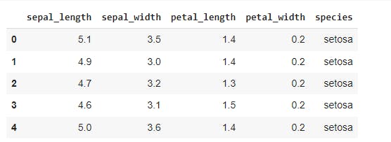
Now, let's run through our dataset:

df=sns.load_dataset('iris')
df.head()

Our dataset is:

First let's find the entropy of each target variable:

def find_entropy(df):
    Class = df.keys()[-1]   #To make the code generic, changing target variable class name
    entropy = 0
    values = df[Class].unique()
    for value in values:
        fraction = df[Class].value_counts()[value]/len(df[Class])
        entropy += -fraction*np.log2(fraction)
    return entropy

Finding the entropy of each attribute..

#entropy of each attriburte

def ent(df,attribute):
    target_variables = df.species.unique()  #This gives all unique species
    variables = df[attribute].unique()
    print(variables)   #This gives different features in that attribute (like 'Sweet')
    entropy_attribute = 0
    for variable in variables:
        entropy_each_feature = 0
        for target_variable in target_variables:
            num = len(df[attribute][df[attribute]==variable][df.species ==target_variable]) #numerator
            den = len(df[attribute][df[attribute]==variable])  #denominator
            fraction = num/(den+eps)  #pi
            entropy_each_feature += -fraction*log(fraction+eps) #This calculates entropy for one feature like 'Sweet'
        fraction2 = den/len(df)
        entropy_attribute += -fraction2*entropy_each_feature   #Sums up all the entropy ETaste

    return(abs(entropy_attribute))

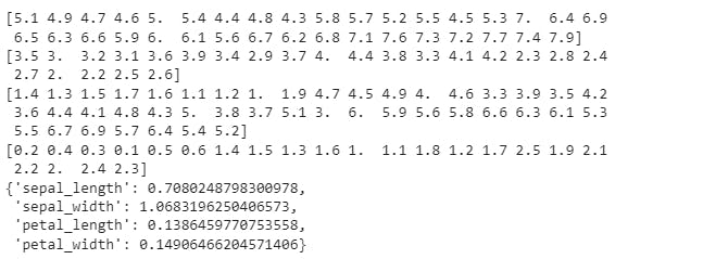
a_entropy = {k:ent(df,k) for k in df.keys()[:-1]}
a_entropy

Output:

Now, it's the time to find the information gain.

def find_IG(df):
    Entropy_att = []
    IG = []
    for key in df.keys()[:-1]:
         #Entropy_att.append(find_entropy_attribute(df,key))
        IG.append(find_entropy(df)-ent(df,key))
    return df.keys()[:-1][np.argmax(IG)]

Generating Tree

def get_subtable(df, node,value):
  return df[df[node] == value].reset_index(drop=True)


def buildTree(df,tree=None): 
    Class = df.keys()[-1]   #To make the code generic, changing target variable class name

    #Here we build our decision tree

    #Get attribute with maximum information gain
    node = find_IG(df)

    #Get distinct value of that attribute e.g Salary is node and Low,Med and High are values
    attValue = np.unique(df[node])

    #Create an empty dictionary to create tree    
    if tree is None:                    
        tree={}
        tree[node] = {}

   #We make loop to construct a tree by calling this function recursively. 
    #In this we check if the subset is pure and stops if it is pure. 

    for value in attValue:

        subtable = get_subtable(df,node,value)
        clValue,counts = np.unique(subtable['species'],return_counts=True)                        

        if len(counts)==1:#Checking purity of subset
            tree[node][value] = clValue[0]                                                    
        else:        
            tree[node][value] = buildTree(subtable) #Calling the function recursively 

    return tree

Build a tree

t=buildTree(df)

Output:

[5.1 4.9 4.7 4.6 5.  5.4 4.4 4.8 4.3 5.8 5.7 5.2 5.5 4.5 5.3 7.  6.4 6.9
 6.5 6.3 6.6 5.9 6.  6.1 5.6 6.7 6.2 6.8 7.1 7.6 7.3 7.2 7.7 7.4 7.9]
[3.5 3.  3.2 3.1 3.6 3.9 3.4 2.9 3.7 4.  4.4 3.8 3.3 4.1 4.2 2.3 2.8 2.4
 2.7 2.  2.2 2.5 2.6]
[1.4 1.3 1.5 1.7 1.6 1.1 1.2 1.  1.9 4.7 4.5 4.9 4.  4.6 3.3 3.9 3.5 4.2
 3.6 4.4 4.1 4.8 4.3 5.  3.8 3.7 5.1 3.  6.  5.9 5.6 5.8 6.6 6.3 6.1 5.3
 5.5 6.7 6.9 5.7 6.4 5.4 5.2]
[0.2 0.4 0.3 0.1 0.5 0.6 1.4 1.5 1.3 1.6 1.  1.1 1.8 1.2 1.7 2.5 1.9 2.1
 2.2 2.  2.4 2.3]
[6.4 5.7 5.6 6.2 6.  5.4 4.9]
[3.2 2.8 3.  2.2 2.9 3.4 2.5]
[4.5]
[1.5 1.3 1.6 1.7]
[5.9 6.8 6.2 6. ]
[3.2 2.8 3. ]
[4.8]
[1.8 1.4]
[6.9 6.3 5.6 6.1]
[3.1 2.5 2.8 2.7 3. ]
[4.9]
[1.5 2.  1.8]
[6.7 5.7 6.  6.3]
[3.  2.5 2.2]
[5.]
[1.7 2.  1.5 1.9]
[6.  5.8 6.5 6.3 6.9 5.9]
[2.7 3.2 2.8 3.1 3. ]
[5.1]
[1.6 1.9 2.  2.4 1.5 2.3 1.8]

Final decisions:

import pprint
pprint.pprint(t)

Output:

{'petal_length': {1.0: 'setosa',
                  1.1: 'setosa',
                  1.2: 'setosa',
                  1.3: 'setosa',
                  1.4: 'setosa',
                  1.5: 'setosa',
                  1.6: 'setosa',
                  1.7: 'setosa',
                  1.9: 'setosa',
                  3.0: 'versicolor',
                  3.3: 'versicolor',
                  3.5: 'versicolor',
                  3.6: 'versicolor',
                  3.7: 'versicolor',
                  3.8: 'versicolor',
                  3.9: 'versicolor',
                  4.0: 'versicolor',
                  4.1: 'versicolor',
                  4.2: 'versicolor',
                  4.3: 'versicolor',
                  4.4: 'versicolor',
                  4.5: {'sepal_length': {4.9: 'virginica',
                                         5.4: 'versicolor',
                                         5.6: 'versicolor',
                                         5.7: 'versicolor',
                                         6.0: 'versicolor',
                                         6.2: 'versicolor',
                                         6.4: 'versicolor'}},
                  4.6: 'versicolor',
                  4.7: 'versicolor',
                  4.8: {'sepal_length': {5.9: 'versicolor',
                                         6.0: 'virginica',
                                         6.2: 'virginica',
                                         6.8: 'versicolor'}},
                  4.9: {'sepal_width': {2.5: 'versicolor',
                                        2.7: 'virginica',
                                        2.8: 'virginica',
                                        3.0: 'virginica',
                                        3.1: 'versicolor'}},
                  5.0: {'sepal_length': {5.7: 'virginica',
                                         6.0: 'virginica',
                                         6.3: 'virginica',
                                         6.7: 'versicolor'}},
                  5.1: {'sepal_length': {5.8: 'virginica',
                                         5.9: 'virginica',
                                         6.0: 'versicolor',
                                         6.3: 'virginica',
                                         6.5: 'virginica',
                                         6.9: 'virginica'}},
                  5.2: 'virginica',
                  5.3: 'virginica',
                  5.4: 'virginica',
                  5.5: 'virginica',
                  5.6: 'virginica',
                  5.7: 'virginica',
                  5.8: 'virginica',
                  5.9: 'virginica',
                  6.0: 'virginica',
                  6.1: 'virginica',
                  6.3: 'virginica',
                  6.4: 'virginica',
                  6.6: 'virginica',
                  6.7: 'virginica',
                  6.9: 'virginica'}}

This comes to the end of the tutorial